Determinant and Jacobian
Today I started my linear algebra class by motivating the determinant using a little bit of history and applications. In particular I talked about determinant appearing in the change of variables in integration of multivariate functions in calculus: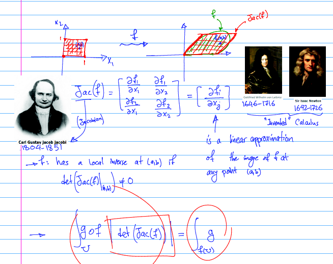 Then after the class I noticed that my picture of what happens when we linearize the image wasn’t very clear as I had drawn it. So I decided to take a look at an actual example. The following code takes a function $f$ that maps $\mathbb{R}^2$ to $\mathbb{R}^2$ and draws three regions:
- the unit cube in blue,
- the image of the unit cube under $f$ in red, and
- the linearization of the image by Jacobian of $f$ at the origin
def show_linearization(f,n=100):
    # f is a function that maps R^2 to R^2 for example
    # f(x,y) = ((x^2+2*(x+2)*(y+1))/4-1,y^2-(x+1)*y)
    # The output is three areas:
        # the unit cube
        # the image of unit cube under f
        # the linearization of the image using the Jacobian of f at (0,0)

    var('x y')
    A = jacobian(f,(x,y))(0,0)
    p = f(0,0)
    domxy = []
    imgxy = []
    jacxy = []
    for i in range(n+1):
        for j in range(n+1):
            domxy.append((i/n,j/n))
            imgxy.append(f(i/n,j/n))
            jacxy.append(p+A*vector([i/n,j/n]))

    P = points(domxy,color="blue",aspect_ratio=1, alpha = .3)
    Q = points(imgxy,color="red",aspect_ratio=1, alpha = .3)
    R = points(jacxy,color="green",aspect_ratio=1, alpha = .3)

    (P+Q+R).show()
Here is a sample run:
f(x,y) = ((x^2+2*(x+2)*(y+1))/4-1,y^2-(x+1)*y)
show_linearization(f)
and the output is:
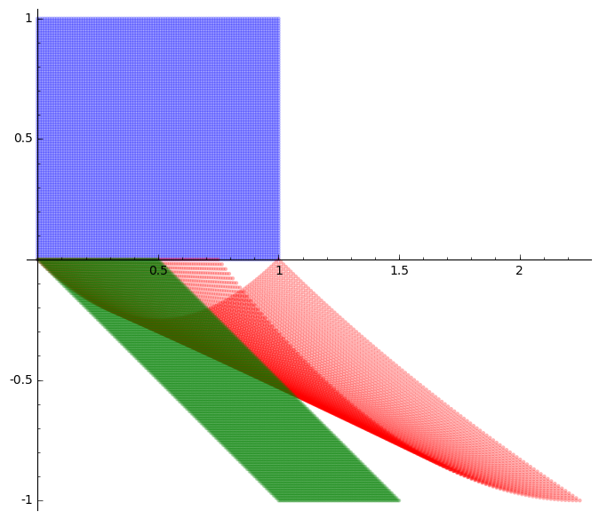
I chose the function in a way that $f(0,0)=(0,0)$ for simplicity. Here it is on sage cell server for you to play around with it: link.
What do you think? Any suggestions or comments?
Leave a comment